Support Vector Machine

See also Support Vector Machine

• Classification
• Supervised
• Non-parametric

Support vector machines are supervised max-margin models with associated learning algorithms that analyze data for classification and regression analysis.

Hard-Margin SVM

Assumption: linear separable

Given $w$, the (signed) distance to the closest example is
$\underset{i\in [n]}{min}\frac{y^{(i)}\cdot w^T{x}^{(i)}}{||w|{|}_2}$

Derivation (distance from a point to a hyperplane)

See also SVM>Margin

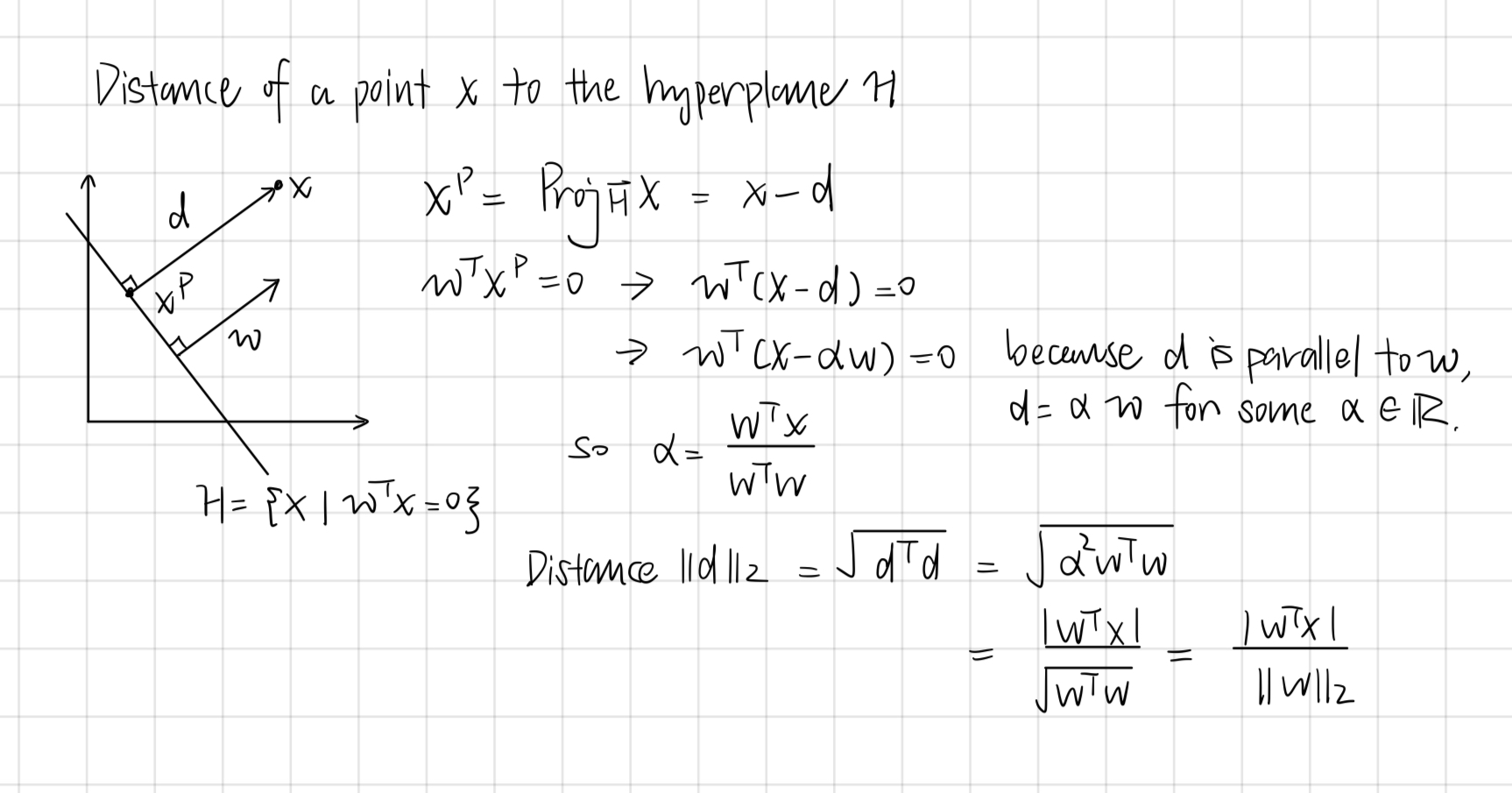
Hence the max-min classifier that maximizes the margin (hard margin) is given by
$\underset{w\in {\mathbb{R}}^d}{max}\underset{i\in [n]}{min}\frac{y^{(i)}\cdot w^T{x}^{(i)}}{||w|{|}_2}$

Because linear separable, we can find $w$ such that $\underset{i}{min}{y}^{(i)}{w}^T{x}^{(i)}=1$
We can fix the scale of $w$ so that $y_i{w}^T{x}_i=1$ for support vectors and $y_i{w}^T{x}_i\ge 1$ for all other points
Therefore it is equivalent to solve the following optimization problem:
$\underset{w\in {\mathbb{R}}^d}{max}\frac{1}{||w|{|}_2}\text{s.t.}{y}^{(i)}\cdot w^T{x}^{(i)}\ge 1,\mathrm{\forall }i\in [n]\to$
$\underset{w\in {\mathbb{R}}^d}{min}\frac{1}{2}||w|{|}_2^2\text{s.t.}{y}^{(i)}\cdot w^T{x}^{(i)}\ge 1,\mathrm{\forall }i\in [n]$

• Is strictly convex
• If a solution exists, then it is unique
• Since we assume the data to be linearly separable, then a solution exists

This is also known as Max-Margin Classifier

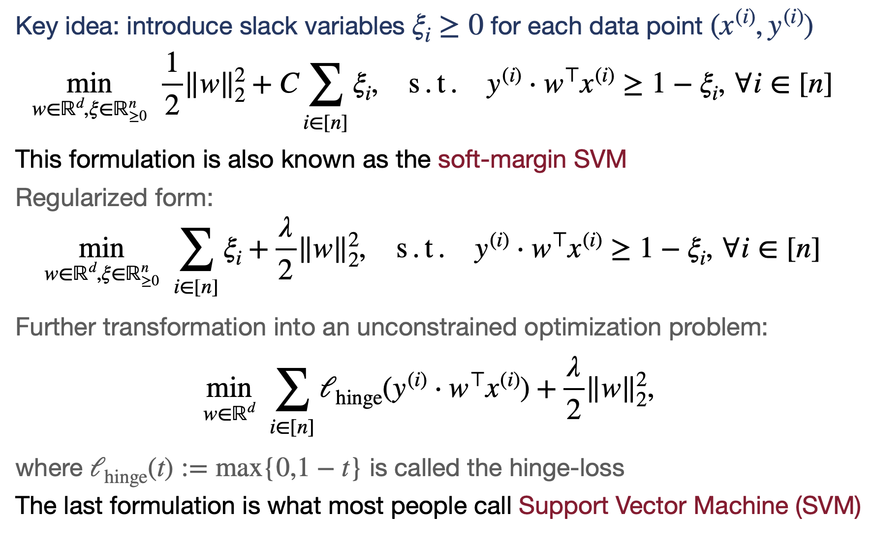
Soft-Margin SVM

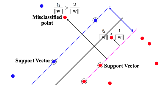
If the data is not linearly separable, we introduce some relaxation through slack variable ${\xi }_i\ge 0$ for each data point $(x^{(i)},y^{(i)})$.

• $1-{\xi }_i\le 0$ means false classification
• $\sum _i{\xi }_i$ is the minimum amount of translation needed to make the optimization problem feasible
• $C$ is a hyper-parameter and $\lambda =\frac{1}{C}$

When we allow misclassifications, the distance between the observations and the threshold is the soft margin. Observations on the edge and within the the soft margin are support vectors.

• If ${\xi }_i=0$, $(x^{(i)},y^{(i)})$ is correctly classified (beyond margin)
• If $0<{\xi }_i\le 1$, $(x^{(i)},y^{(i)})$ is correctly classified (within margin)
• If ${\xi }_i>1$, $(x^{(i)},y^{(i)})$ is wrongly classified

Also known as Support Vector Classifier

Support Vector Machine

Support Vector Machine is Hinge Loss with L2 Regularization

• The loss function is a penalty between a model and the truth
• Regularization is a penalty for too complex model

See also Neural Net#Overfitting

Hinge Loss

$\underset{w\in {\mathbb{R}}^d}{min}\sum _i{\mathcal{L}}_{\text{hinge}}(y^{(i)}\cdot w^T{x}^{(i)})+\frac{\lambda }{2}||w|{|}_2^2$
where ${\mathcal{L}}_{\text{hinge}}(t)=max\{0,1-t\}$

Derivation:
Further transformation into an unconstrained optimization problem

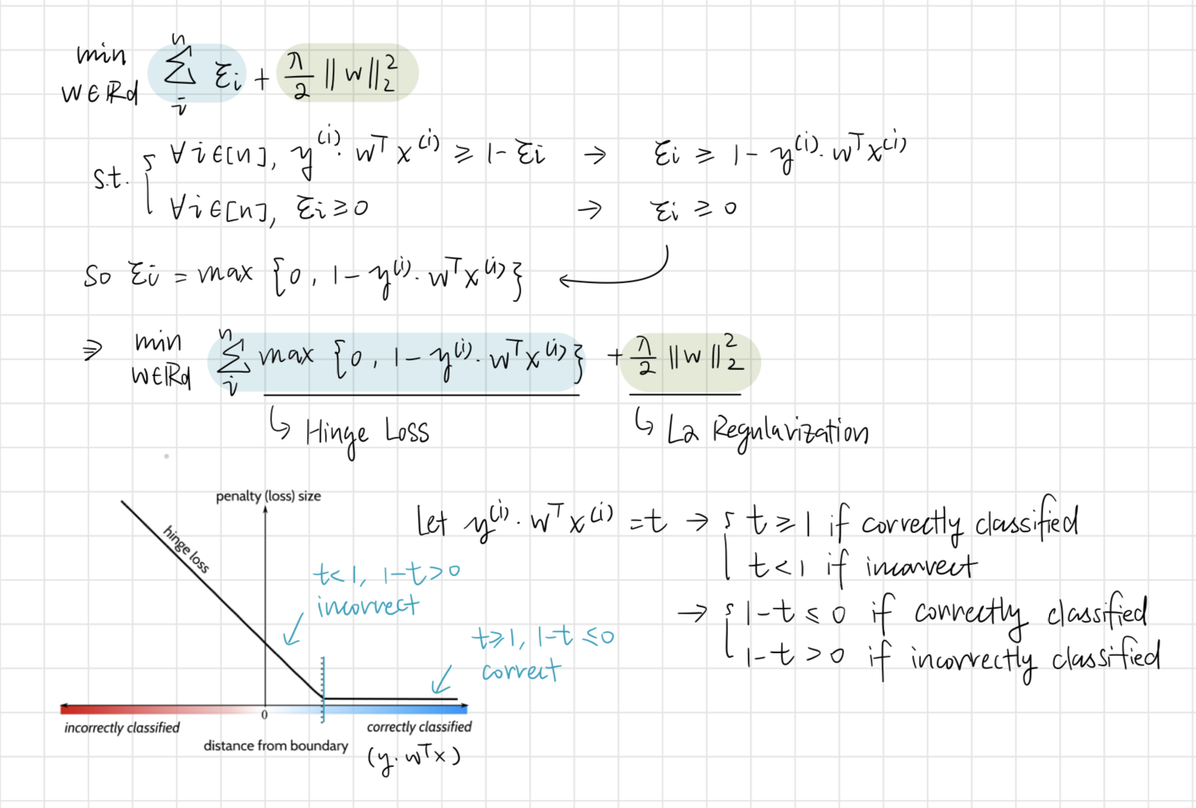
The hyper-parameter $\lambda \ge 0$ controls the strength of regularization:

• If $\lambda \to 0$, then less focus on regularization, more focus on loss
• If $\lambda \to \mathrm{\infty }$, then more focus on regularization, less focus on loss

Dual SVM

In Hard-Margin SVM:
We introduce ${\alpha }_i\ge 0$ for each of the constraint in $\underset{w\in {\mathbb{R}}^d}{min}\frac{1}{2}||w|{|}_2^2\text{s.t.}{y}^{(i)}\cdot w^T{x}^{(i)}\ge 1,\mathrm{\forall }i\in [n]$
$\underset{w}{min}\underset{\alpha }{max}\mathcal{L}(w,\alpha )=\frac{1}{2}||w|{|}_2^2+\sum _i{\alpha }_i(1-y^{(i)}\cdot w^T{x}^{(i)})$
(the Lagrangian)

• ${\alpha }_i$ - the price to pay if the corresponding constraint is violated
• Transform into unconstrained problem
• Two cases (because we are trying to find $\alpha$ to maximize the equation):
  • If $i$th constraint holds, $1-y^{(i)}\cdot w^T{x}^{(i)}\le 0$ then ${\alpha }_i^{\ast }=0$
  • If $i$th constraint is violated, $1-y^{(i)}\cdot w^T{x}^{(i)}>0$ then ${\alpha }_i^{\ast }\to \mathrm{\infty }$

$\underset{w}{min}P(w)=\underset{\alpha }{max}D(\alpha )$ where we define

• Primal Problem $P(w)=\underset{\alpha }{max}\mathcal{L}(w,\alpha )$
• Dual Problem $D(\alpha )=\underset{w}{min}\mathcal{L}(w,\alpha )$

This is because of Strong Duality:

• In general, for an arbitrary function $f(x,y)$, we have weak duality
  $\underset{x}{min}\underset{y}{max}f(x,y)\ge \underset{y}{max}\underset{x}{min}f(x,y)$
• For convex problems with affine constraints, we have strong duality
  $mi{n}_x\underset{y}{max}f(x,y)=\underset{y}{max}\underset{x}{min}f(x,y)$

The Dual Problem

The dual problem $D(\alpha )=\underset{w}{min}\mathcal{L}(w,\alpha )$ is solvable due to convexity
$\underset{\alpha }{max}D(\alpha )=\sum _i{\alpha }_i-\frac{1}{2}\sum _{i,j}{\alpha }_i{\alpha }_j{y}_i{y}_j{x}_i^T{x}_j=1_n^T\alpha -\frac{1}{2}{\alpha }^{T}K\alpha$
where $1_n\in {\mathbb{R}}^n$ is all-one vector of dim-$n$ and $K\in {\mathbb{R}}^{n\times n}$ with $K_{ij}=(y_i{x}_i{)}^T(y_j{x}_j)$

• The optimization $\underset{\alpha }{max}D(\alpha )$ wrt $\alpha$ is a quadratic program
• Solve for ${\alpha }^{\ast }$
• Recover the optimal $w^{\ast }$ with $w^{\ast }=\sum _i{\alpha }_i^{\ast }{y}^{(i)}{x}^{(i)}$
  • The optimal normal vector $w^{\ast }$ is a linear combination of $y^{(i)}{x}^{(i)}$
  • Only the ones with ${\alpha }_i^{\ast }>0$ contributes to $w^{\ast }$
  • The ones with ${\alpha }_i^{\ast }=0$ does not contribute to $w^{\ast }$
  • The points $y^{(i)}{x}^{(i)}$ with ${\alpha }_i^{\ast }>0$ are support vectors
  • ${\alpha }_i^{\ast }>0\to y^{(i)}{w}^T{x}^{(i)}=1$

Dual solutions and support vectors are not necessarily unique
(even if the primal solution is unique)

Derivation:

The Dual Problem makes #Kernel Method easier

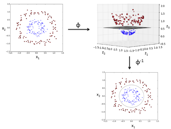
Kernel Method

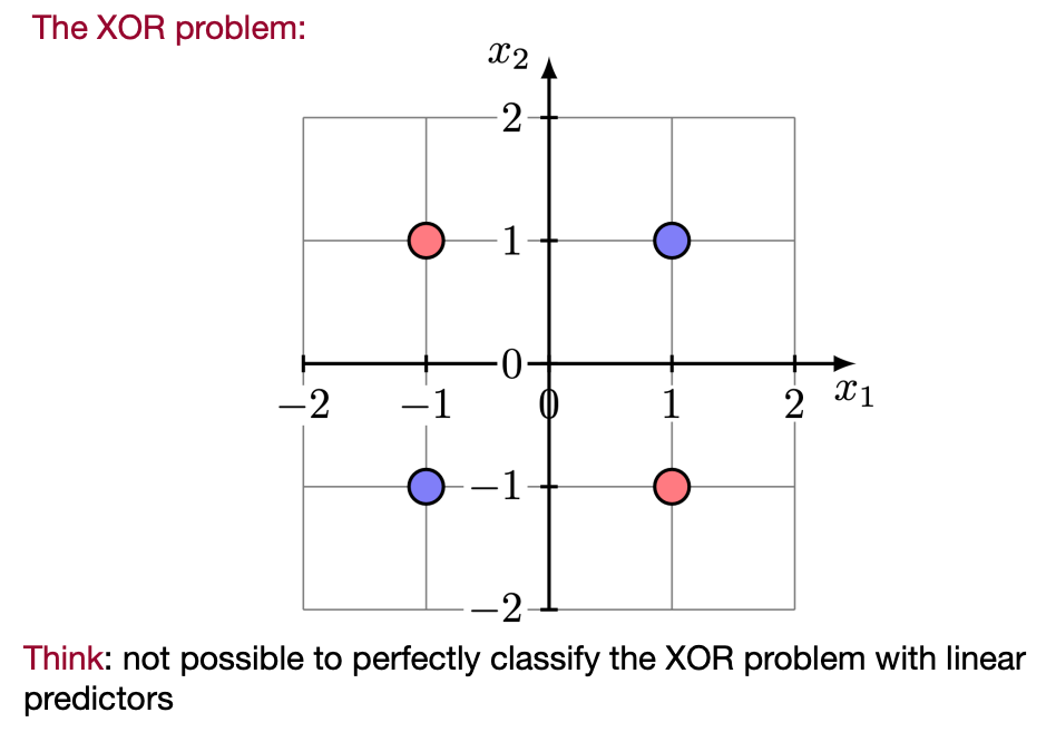
Sometimes datasets are linearly inseparable, in which case we use the Kernel Method.
Key idea is feature mapping/lifting to construct new features.
$\varphi (\cdot ):{\mathbb{R}}^d\to {\mathbb{R}}^p$

Example:
In the XOR Problem, we can add a third dimension $(x_1,x_2)\to (x_1,x_2,x_3)$
where $x_3=x_1{x}_2$

The primal optimization becomes $\underset{w\in {\mathbb{R}}^d}{min}\frac{1}{2}||w|{|}_2^2\text{s.t.}{y}^{(i)}\cdot w^T\varphi (x^{(i)})\ge 1,\mathrm{\forall }i\in [n]$
#The Dual Problem under the feature map $\varphi$ is therefore
$\underset{\alpha }{max}D(\alpha )=\sum _i{\alpha }_i-\frac{1}{2}\sum _{i,j}{\alpha }_i{\alpha }_j{y}_i{y}_j\varphi (x_i{)}^T\varphi (x_j)=1_n^T\alpha -\frac{1}{2}{\alpha }^{T}K\alpha$
where $1_n\in {\mathbb{R}}^n$ is an all-one vector of dimension $n$ and $K\in {\mathbb{R}}^{n\times n}$ with $K_{ij}=(y_i\varphi (x_i){)}^T(y_j\varphi (x_j))$

• The dual form never needs $\varphi (x)\in {\mathbb{R}}^p$ explicitly, but only the inner product $\varphi (x{)}^T\varphi (x^{\prime })\in \mathbb{R}$
• Kernel Trick: Replace every $\varphi (x{)}^T\varphi (x^{\prime })$ with kernel evaluation $k(x,x^{\prime })$
  • Sometimes $k(x,x^{\prime })$ is much cheaper
  • But we need to explicitly maintain $K\in {\mathbb{R}}^{n\times n}$

Example:
Affine features $\varphi :{\mathbb{R}}^d\to {\mathbb{R}}^{d+1}$ with
$\varphi (x)=(1,x_1,...,x_d)$
The kernel form is $\varphi (x{)}^T\varphi (x^{\prime })=1+x^T{x}^{\prime }$

Quadratic features $\varphi :{\mathbb{R}}^d\to {\mathbb{R}}^p$ with
$\varphi (x)=(x_1^2,x_2^2,\sqrt{2}{x}_1{x}_2,\sqrt{2}{x}_1,\sqrt{2}{x}_2,1)$
The kernel form is $\varphi (x{)}^T\varphi (x^{\prime })=(1+x^T{x}^{\prime }{)}^2$

RBF Kernel

Radial Basis Function (RBF/Gaussian) Kernel
For any $\sigma >0$, there is an infinite-dim feature map $\varphi :{\mathbb{R}}^d\to {\mathbb{R}}^{\mathrm{\infty }}$ such that
$k(x,x^{\prime })=\varphi (x{)}^T\varphi (x^{\prime })=exp(-\frac{||x-x^{\prime }|{|}_2^2}{2{\sigma }^2})$